Over-concentration in glycol loops: what the reference data shows
A worked analysis of concentration, freezing point and viscosity in a glycol loop, with the pumping-energy penalty of over-concentrating expressed as a range.
THE SHORT ANSWER
What you need to know.
Freeze protection is chosen against a worst case while pumping energy is paid continuously, so glycol loops tend to be over-concentrated. The reference series for the glycol-type range quantifies it. Freezing point improves 41 K between 20 and 60 wt%, then stops being tabulated as a value, and above 45 wt% the top of the series is weakest. At fixed duty the effects compound: flow rises by a quarter and viscosity multiplies by eight. The pumping penalty is +244% if both charges stay turbulent, +1229% if both are laminar, and as little as +110% if they sit either side of the transition.
- Freezing point improves steeply to about 60 wt%, then stops being tabulated as a value, and the 90 wt% point is the weakest figure above 45 wt%.
- At a common temperature, viscosity rises far faster with concentration than freeze protection improves.
- At a fixed duty the two penalties compound — a more concentrated charge both carries less heat per litre and is harder to pump.
1. The decision, and why it is usually made conservatively
A water-diluted glycol coolant is specified by concentration. That single number fixes three things at once: the temperature below which the fluid freezes, its viscosity at every operating temperature, and — through viscosity — the pumping energy the loop will consume for its entire service life.
The first of those is a safety property, and it is the one that tends to drive the decision. Freeze protection is sized against a worst case, and worst cases are naturally specified with margin. The second and third are running costs, and running costs do not fail dramatically. The result is a systematic bias: loops are concentrated for a freeze event that will probably never occur, and the pump pays for that margin every hour.
The bias is worth quantifying rather than deploring. The reference data for the glycol-type range is sufficient to do it, and the answer turns out to be larger than most specifications assume.
2. Data and method
All product figures below are the reference values published in the 21 August 2026 edition of the Glacier Coolant product data. That is the only version used, and the conclusions are tied to it.
Data. The concentration series used here is the reference data for the LM-4 range — a glycol-type (modified-diol) heat transfer fluid specified across −35 °C to +150 °C depending on model. It reports, for each concentration, the density at 20 °C, the freezing point, and a viscosity figure with the temperature at which it was measured:
| Concentration (wt%) | Density at 20 °C (g/cm³) | Freezing point (°C) | Viscosity (cP) | measured at |
|---|---|---|---|---|
| 20 | 1.024 | −8.0 | 2.45 | +5 °C |
| 25 | 1.032 | −11.0 | 3.25 | 0 °C |
| 30 | 1.038 | −15.0 | 5.49 | −5 °C |
| 35 | 1.048 | −19.0 | 7.93 | −10 °C |
| 40 | 1.058 | −23.0 | 12.37 | −15 °C |
| 45 | 1.062 | −29.0 | 18.94 | −20 °C |
| 50 | 1.066 | −35.0 | 32.90 | −25 °C |
| 55 | 1.072 | −42.0 | 53.57 | −30 °C |
| 60 | 1.078 | −49.0 | 63.63 | −30 °C |
| 70 | 1.089 | < −45.0 | 51.96 | −20 °C |
| 80 | 1.101 | < −45.0 | 70.20 | −20 °C |
| 90 | 1.113 | −29.5 | 65.03 | −10 °C |
The measurement-temperature column is the whole difficulty. Viscosity is strongly temperature-dependent, and the series pairs each concentration with a temperature close to that concentration's own freezing point — from +5 °C at 20 wt% down to −30 °C at 55 and 60 wt% — though the three highest concentrations are measured at −20, −20 and −10 °C, which does not follow the same pattern. Read the viscosity column top to bottom and it rises, with two dips — at 70 and 90 wt% — that are themselves a clue; read it with the temperature column and the apparent pattern falls apart, because the rows describe different operating points rather than one fluid at one temperature.
Any comparison that ignores this is meaningless. The comparison here therefore uses only pairs at a common temperature. The series supports five such pairs across three temperatures: 55 and 60 wt% at −30 °C; 45, 70 and 80 wt% at −20 °C; and 35 and 90 wt% at −10 °C.
Two further figures come from outside the concentration table. Specific heat is given at 0.837 cal/g·°C for a 35 wt% charge at an operating temperature of −10 °C, in a comparison of secondary refrigerants at a matched freezing point, and at 0.619 cal/g·°C for the stock solution at 20 °C, in the description of the series itself. The stock-solution density is quoted there as a range, 1.105 to 1.125 g/cm³; the 90 wt% row of the concentration table, at 1.113 g/cm³, is taken as the point value.
Method. Three relations are used, all standard:
- Volumetric heat capacity — the energy a litre carries per kelvin — is the product of density and specific heat. The two specific-heat points above are used, and the intermediate values required for section 6 are linearly interpolated between them.
- Volumetric flow for a given duty follows as V̇ = Q / (ρ · c_p · ΔT).
- Pumping power for fixed pipework scales with viscosity and velocity through the friction factor. In fully laminar flow, pressure drop is proportional to μ·v; in turbulent flow following the Blasius correlation it scales as ρ^0.75 · μ^0.25 · v^1.75. Because a change in concentration changes both viscosity and — at fixed duty — velocity, both are carried through the calculation in section 6.
3. Result one: the freeze-protection curve stops paying
The freezing point improves steeply up to about 60 wt%. Beyond that the series stops quoting a value for 70 and 80 wt%, and the next figure it gives is the 90 wt% point:
| Interval | Change in freezing point |
|---|---|
| 20 → 30 wt% | 7.0 K lower |
| 30 → 40 wt% | 8.0 K lower |
| 40 → 50 wt% | 12.0 K lower |
| 50 → 60 wt% | 14.0 K lower |
| 60 → 70 wt% | not resolvable — reported only as a bound |
| 70 → 80 wt% | not resolvable — reported only as a bound |
| 60 → 90 wt% | 19.5 K higher — the freezing point gets worse |
Three findings follow, and each matters more than the smooth curve suggests.
Each additional point of concentration buys more protection, up to a limit. The gain per five percentage points rises from about 3 K near the bottom of the series to 7 K near the top. That is the useful part of the curve, and it is the reason a modest increase in concentration is often justified.
The last interval is not quantified. At 70 and 80 wt% the freezing point is reported only as below −45 °C — a bound rather than a value. Whatever protection those concentrations add cannot be established from the series, which is itself an argument against specifying them: a concentration whose benefit is not stated is a concentration whose cost cannot be justified against it. Note also that the 60 wt% point is tabulated at −49.0 °C, which is below the bound given for 70 and 80 wt%; the series is not internally consistent in that region, and it should be treated as a gap rather than read as a plateau.
Above 45 wt%, the top of the series is its weakest point. The 90 wt% figure is −29.5 °C, which is above the 50 wt% point at −35.0 °C and above the 55, 60, 70 and 80 wt% points as well. It is not weaker than everything in the series — the 20 to 45 wt% points are all warmer than it — but it is the worst figure in the upper half of the range. That reversal should be read with one caution attached. It is a single tabulated figure, and it sits beside a description of the stock solution as freezing below −50 °C; the two are not easily reconciled. The practical conclusion does not depend on it: the argument against the top of the series rests on 70 and 80 wt%, where the freezing point is already unquantified and, within the −20 °C group, viscosity is the highest of the three concentrations measured there.
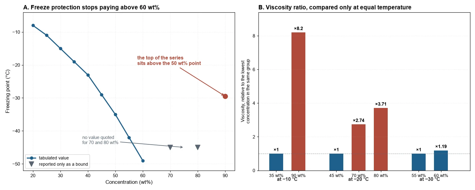
Both effects are visible when the series is plotted. The freezing point falls steeply to about 60 wt%, then stops being reported as a value, and the single figure available at the top of the series sits above the 50 wt% point. The second panel shows why the concentration decision matters more than that reversal. At each common temperature, viscosity climbs steeply with concentration — and the concentrations at the top of the series, where freeze protection has stopped being quantified, are the ones carrying the largest viscosity penalty at the temperature where they would actually run.
4. Result two: at a common temperature, viscosity rises far faster
This is where the cost of the margin appears. Holding temperature constant:
| Common temperature | Concentrations compared | Viscosity ratio |
|---|---|---|
| −30 °C | 55 wt% (53.57 cP) → 60 wt% (63.63 cP) | ×1.19 |
| −20 °C | 45 wt% (18.94 cP) → 70 wt% (51.96 cP) | ×2.74 |
| −20 °C | 70 wt% (51.96 cP) → 80 wt% (70.20 cP) | ×1.35 |
| −20 °C | 45 wt% (18.94 cP) → 80 wt% (70.20 cP) | ×3.71 |
| −10 °C | 35 wt% (7.93 cP) → 90 wt% (65.03 cP) | ×8.20 |
The −20 °C set is the most instructive, because all three concentrations are measured at the same temperature. Moving from 45 to 80 wt% multiplies viscosity by 3.71, and the freezing point moves from −29.0 °C to something below −45 °C.
Whether that trade is justified depends entirely on the duty. If the loop must survive −40 °C, the 45 wt% charge freezes and there is no decision to make. If the loop's coldest condition is −25 °C, the 45 wt% charge already covers it with 4 K of margin, and the 80 wt% charge buys protection that will never be called upon while multiplying viscosity by 3.71 at the one temperature where the two are directly comparable.
5. Result three: what the viscosity ratio does to pumping power
For fixed pipework, a pumping penalty follows from the viscosity ratio and the flow regime. The table below holds the flow constant, which isolates the viscosity effect; section 6 then adds the second effect that a real fixed duty produces:
| Case | Viscosity ratio | Penalty, turbulent bound (viscosity term alone) | Penalty, laminar bound (μ^1.0) |
|---|---|---|---|
| 55 → 60 wt% at −30 °C | ×1.19 | +4% | +19% |
| 45 → 80 wt% at −20 °C | ×3.71 | +39% | +271% |
| 35 → 90 wt% at −10 °C | ×8.20 | +69% | +720% |
The width of that range is the honest answer, and the two ends describe different plants. The turbulent column shows the viscosity contribution alone; because density also rises slightly with concentration, the full fixed-flow turbulent figure at this viscosity ratio is +77% rather than +69%.
The 55 to 60 wt% case is the one most specifications will recognise. It is a modest over-concentration — the kind produced by rounding a requirement up to the next familiar figure — and at a common −30 °C it costs between 4% and 19% in pumping power. That is not dramatic, and it is the true scale of the problem for most loops.
The 45 to 80 wt% case is the deep-cryo decision, and it is where the arithmetic becomes large. A loop that must survive below −45 °C has no choice; a loop whose coldest condition is −25 °C and which nevertheless carries an 80 wt% charge is paying 39% to 271% for protection it will never use.
Both cases above are quoted on the viscosity term alone. Adding the density contribution as section 6 does raises each turbulent figure by roughly a tenth again.
The second case is the more eye-catching, and the first is the more common. A specification is far more likely to be over-concentrated by five percentage points than by thirty-five.
Three qualifications matter as much as the numbers, and the first is the most consequential.
A fixed-speed pump does not hold flow constant. The table above answers the question "what does it cost to move the same volume?" That is not what a real installation does. Change the concentration and the pump stays as it is, running at the same speed. On its curve, a higher system resistance moves the operating point to lower flow — so the pump power changes far less than the hydraulic prediction, and the loss appears somewhere else: as reduced volumetric flow, a wider temperature rise across the load, and a process temperature that can no longer be held.
The +271% figure should therefore be read as "moving this flow at this concentration requires a different pump or larger pipework" rather than as an electricity bill. That reading is arguably more serious, because the consequence is lost cooling capacity rather than a larger invoice — and it will not be discovered until the plant is asked to perform at design conditions. Where a measured pump power draw exists at both concentrations, that measurement supersedes both bounds, because it already contains the operating-point shift.
The exponent band is not a sealed wall. The fourth-root limit assumes smooth pipework and fully turbulent flow. Two effects push against it in opposite directions. At high Reynolds numbers in rough commercial pipe, the friction factor becomes independent of Reynolds number, the viscosity exponent tends toward zero, and the penalty is smaller than the table suggests. In the transitional band around Reynolds numbers of 2,300 to 4,000, the local exponent is steeper than a quarter, and the penalty is larger. Cold secondary loops with glycol commonly operate in or near that transitional band, which is one reason the spread between the two bounds is wide rather than merely cautious. Fittings and heat exchangers add a further pressure loss that varies with velocity squared and not with viscosity at all, which pushes the effective exponent lower again.
The regime shifts as concentration rises. The bounds treat the regime as fixed, but viscosity determines the regime: as a fluid becomes more viscous, the Reynolds number for a given flow falls, and a loop that was turbulent at low concentration can become laminar at high concentration. Worked through for a DN50 line at 1.5 m/s and −20 °C, taking the bore as 52.5 mm, the 45 wt% charge sits at a Reynolds number of roughly 4,400 — marginally turbulent — while the 80 wt% charge falls to about 1,200, which is comfortably laminar. The transition is not a marginal one. The laminar column is therefore not a theoretical case for an over-concentrated loop; it is where the loop ends up.
6. Result four: the second penalty, and why it does not offset the first
There is a second mechanism, and it points the same way as the first rather than against it.
Density rises with concentration — from 1.024 to 1.113 g/cm³ across the series, about 8.7% — and taken alone that would be mildly helpful, because a denser fluid carries the same mass flow in less volume. Specific heat falls faster in the opposite direction. The two available data points are 0.837 cal/g·°C for a 35 wt% charge and 0.619 cal/g·°C for the stock solution at the top of the series: a fall of 26%, against a density rise of 6% over the same interval.
Volumetric heat capacity — the product of the two — therefore falls, and the flow required for a fixed duty rises with it:
| Concentration | Density (g/cm³) | Specific heat (cal/g·°C) | Volumetric heat capacity (MJ/m³·K) | Flow for 100 kW at ΔT = 5 K |
|---|---|---|---|---|
| 35 wt% | 1.048 | 0.837 | 3.67 | 5.45 L/s |
| 50 wt% | 1.066 | 0.778 | 3.47 | 5.77 L/s |
| 80 wt% | 1.101 | 0.659 | 3.03 | 6.59 L/s |
| 90 wt% (top of series) | 1.113 | 0.619 | 2.88 | 6.94 L/s |
A loop asked to carry the same duty at higher concentration has to move more volume, not less — about 21% more at 80 wt% than at 35 wt%, and 27% more at 90 wt%. The density effect does not offset the viscosity penalty; the two compound, because the same charge makes the fluid both harder to pump and less able to carry heat per litre.
This changes the pumping arithmetic materially, and in the direction of a larger penalty. Section 5 held the flow constant to isolate the viscosity effect, which is the right way to separate the mechanisms — but it is not what a real loop does.
At fixed duty, velocity rises along with flow. Pumping power is the product of volumetric flow and pressure drop, P = V̇ · Δp, and V̇ is proportional to velocity in a fixed pipe — so the velocity exponent in the power law is one higher than the exponent in the pressure-drop relation. Section 2 gave Δp ∝ μ·v for laminar flow and Δp ∝ ρ^0.75 · μ^0.25 · v^1.75 for turbulent flow; multiplying each by the flow term gives:
- laminar: P ∝ μ · v²
- turbulent: P ∝ ρ^0.75 · μ^0.25 · v^2.75
That extra power of velocity is what makes the fixed-duty penalty so much larger than the fixed-flow one, and it is the step most easily dropped when the two are compared. Substituting the ratios from this case — density ×1.062, viscosity ×8.20, velocity ×1.273:
| Case (35 → 90 wt% at −10 °C) | Flow | Viscosity | Pumping power, turbulent | Pumping power, laminar |
|---|---|---|---|---|
| Fixed flow (isolates viscosity) | ×1.00 | ×8.20 | +69% | +720% |
| Fixed duty, both ends turbulent | ×1.27 | ×8.20 | +244% | — |
| Fixed duty, both ends laminar | ×1.27 | ×8.20 | — | +1229% |
| Fixed duty, mixed regimes (lean turbulent, concentrated laminar) | ×1.27 | ×8.20 | +435% → +110% | — |
The first two fixed-duty rows assume both charges sit in the same flow regime. Section 5 showed that they need not: the concentrated charge becomes laminar while the lean one is still turbulent. Because the ratio of the two Reynolds numbers is fixed by the fluid properties — here about 0.16 — there is a band of loop conditions in which the lean charge is turbulent and the concentrated charge is already laminar. In that band the penalty runs from about +435% down to about +110% as flow increases.
That makes +110%, not +244%, the bottom of the envelope. The +244% figure is what a loop that stays fully turbulent at both concentrations pays; a loop sitting between the regimes pays less, because the concentrated charge gains the laminar pressure-drop relation while the lean one does not.
On the turbulent bound the extra pumping power is about 3.2 times larger under the fixed-duty framing, from +77% to +244%; on the laminar bound the effect is smaller, raising it from +720% to +1229%. Which bound applies depends on the loop's Reynolds number, which the loop geometry and the fluid together determine. The reason is that the two changes are not independent: a fluid that carries less heat per litre must circulate faster, and circulating a more viscous fluid faster is progressively more expensive.
7. Applying it: an audit before the next fill
A procedure that takes an afternoon and can be run against an existing specification follows from the above.
- Establish the coldest fluid condition, not the process setpoint — and be specific about which fluid condition. The bulk fluid temperature at the coldest point and the temperature at the evaporator wall or film are not the same, and the difference is often several kelvin. Since each kelvin of freezing point is worth roughly 0.7 to 0.8 percentage points of concentration in the steep part of the curve, that ambiguity can consume the entire margin being evaluated. State which one the requirement refers to, and size the concentration against it. Include pull-down, defrost, standby and any part of the circuit exposed to ambient in winter.
- Read the concentration that the freezing point requires, interpolating between table rows rather than rounding upward. Interpolating between 45 and 50 wt% is legitimate; rounding to 60 wt% "for safety" is not, because it is not safety that is being purchased.
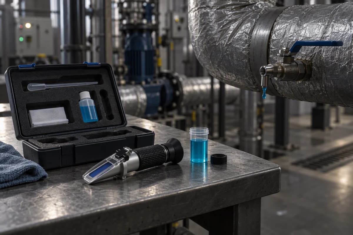
- Check the concentration actually in the loop. A refractometer reading against a calibration curve for the specific product takes minutes, and it is the only reliable way to know what is actually in the loop. A specification and a plant rarely agree by accident.
- Compare viscosity at the loop's real operating temperature, using the same-temperature figures rather than the tabulated column.
- Estimate the pumping penalty using the two bounds, and check which regime the loop is in. If the pump has a measured power draw at the current concentration, that measurement beats both bounds.
8. Limitations
Several constraints apply, stated so that the conclusions can be weighed rather than merely accepted.
Specific heat is tabulated at only two points, and neither is in the concentration series. The 0.837 cal/g·°C figure is for a 35 wt% charge at an operating temperature of −10 °C, and the 0.619 figure is for the stock solution at 20 °C. The 50 and 80 wt% values used in section 6 are linear interpolations between them, and the true curve need not be linear. The two endpoints are also quoted at different temperatures, while the densities they are multiplied by are both at 20 °C. The direction of the effect is not in doubt — specific heat falls by 26% across the interval — but the intermediate figures are approximate, and this is the largest single source of uncertainty in the result.
The viscosity exponents are bounds, not measurements. The fourth-root and first-power limits are textbook results for fully turbulent and fully laminar flow in smooth pipework. Real loops have fittings and heat exchangers whose pressure loss is largely independent of viscosity, which pushes the effective exponent below a quarter, alongside fouling, which pushes it up. No specific loop's penalty is claimed.
Viscosity is reported at one temperature per concentration. The series does not provide a full viscosity-temperature matrix for a single concentration, which is why only common-temperature comparisons are used. Five such comparisons exist and all five are used.
The heat-exchanger side is not analysed here, and for a cold loop it may be the larger effect. Viscosity does not only raise pressure drop; it lowers the Reynolds number, and a lower Reynolds number reduces the tube-side heat transfer coefficient. In an evaporator, that shows up as a wider approach: with a lower coefficient, the gap between the fluid being cooled and the evaporating refrigerant has to widen for the same heat to move, so the evaporating temperature runs colder and the compressor works at a lower suction temperature for the same delivered duty — an energy penalty on the refrigeration side rather than the circulation side. For a loop at −28 °C with an 80 wt% charge already in laminar flow, that penalty can exceed the pumping penalty calculated above, and in a cold loop it may be the dominant one. One of the two cost mechanisms is covered here, and for a cold loop the other can be the larger one.
The chemistry is described by family, not by name. The series is described as glycol-type modified diols. The freezing-point behaviour in section 3, including the reversal at the top of the series, is characteristic of the concentration curve for the specific glycol in use, and other glycol chemistries do not necessarily behave the same way. The figures are the ones published for this product and should not be transferred to a different glycol without checking that product's own series.
A second concentration series exists in the same document, and it suggests the specific-heat fall may be steeper than the linear interpolation used here. The LM-4B series tabulates specific heat at two concentrations. Its table labels the column as cal/g·°C, but the values given — 3.190 and 2.611 — cannot be in that unit, since water itself is 1.0; read as kJ/(kg·K), which the magnitudes fit, they convert to roughly 0.762 cal/g·°C at 40 wt% and 0.624 at 50 wt%. That is a steeper fall than the straight line drawn between the two points used in section 6, though the comparison is between a ten-point interval and a fifty-five-point one, so the slopes are not directly comparable. The two points are also measured at different temperatures, −10 and −20 °C, which is the same objection raised against section 6 above. It is a different formulation and its figures cannot be substituted directly, but the direction of the difference matters: it means the flow increase calculated here is more likely to be an underestimate than an overestimate.
The freezing-point determination method is not stated. Freezing points are measured by methods that differ in how they treat supercooling, and the figures tabulated here do not say which was used. For the comparisons used above that does not matter, because all rows come from one series measured the same way. It would matter if these figures were compared against a determination made by a different method.
Purchase cost is not included. Concentration is also a consumable, and a loop filled at 80 wt% contains substantially more concentrate than the same loop at 45 wt% — a cost carried at first fill and at every subsequent top-up. That belongs on the other side of the ledger from the pumping penalty, and it points in the same direction, but it is not quantified here.
No independent measurement was made. All property figures are reference values published by the manufacturer. They are described as reference values, and no independent testing or third-party endorsement is implied. One external cross-check is available and reassuring: the 35 wt% properties used here — density 1.048 g/cm³, specific heat 3.502 kJ/kg·K, viscosity 7.93 cP at −10 °C — agree closely with the independent property data for aqueous ethylene glycol solutions published by the KTH refrigeration group, whose 36 wt% solution gives 7.99 mPa·s at −10 °C, with a specific heat of 3.494 kJ/kg·K at that temperature. Note also that the comparison table gives 6.73 cP for the same 35 wt% charge at −10 °C, where the concentration series gives 7.93 cP: the two do not agree, and the higher, more conservative figure is used above.
One scope note. The argument here concerns over-concentration, not concentration. Nothing suggests reducing concentration below the duty requirement. Freeze protection below the coldest condition is a safety requirement, and the criticism is of margin added beyond it.
9. What would change the conclusion
Four findings would overturn or materially qualify the argument, and each is testable.
A measured pumping penalty that is smaller than the turbulent bound. If a loop's measured pump power at two concentrations differs by less than μ^0.25 predicts, the loops in question are operating in a regime better than Blasius, and the practical cost of margin is correspondingly lower than the range suggests.
A full viscosity-temperature matrix. The ratios above are computed at three temperatures because that is all the series supports. A full matrix would show whether the gaps between concentrations widen or narrow as temperature falls. If they narrow, the penalty is concentrated at the warm end of the operating range and the cold-end figures here overstate the annual cost; if they widen, the opposite.
A freezing-point determination for the 70 and 80 wt% points. If those concentrations were measured to a lower bound and found to deliver materially better protection than 60 wt%, the argument against specifying them would narrow to a cost-versus-benefit question rather than a benefit-free one.
A measured evaporator performance comparison. If a loop's evaporator approach and compressor power were measured at two concentrations and found not to differ, the heat-exchanger mechanism described in the limitations would be shown to be small in that application — which would place the pumping penalty back at the centre of the decision, and make the case for trimming concentration weaker.
10. Conclusion
Concentration is normally set by the freezing point and paid for by the pump. The reference data shows the two moving at very different rates: 40 percentage points of concentration between 20 and 60 wt% buy 41 K of freeze protection, after which the curve stops being reported as a value and the top of the series turns out to be the weakest figure above 45 wt%. At a common temperature, the viscosity multiplier from adding concentration beyond the requirement runs from 1.19 to 8.20 across the cases that can be compared. And because specific heat falls as concentration rises, a loop carrying the same duty has to circulate faster — so the viscosity penalty and the flow penalty compound rather than offset, putting the fixed-duty pumping penalty for the widest comparison at +244% where both concentrations stay turbulent, +1229% in fully laminar flow, and as little as +110% where the two sit on opposite sides of the transition.
The practical conclusion is not that glycol loops should run lean. It is that concentration above the point where freeze protection stops being quantified is bought at the highest viscosity in the temperature group where it runs, and that it is usually added by default rather than by calculation. Reading the concentration the duty actually requires, and measuring the concentration actually in the loop, is the cheapest efficiency measure available in most secondary cooling systems — and it requires no capital expenditure at all.
QUICK CLARIFICATIONS
Common questions.
Why not simply specify the highest concentration available?
Because above about 60 wt% the freezing point stops being reported as a value. The series gives −49 °C at 60 wt%, then reports only a bound at 70 and 80 wt%, and the single figure at 90 wt% sits above the 50 wt% point. A concentration whose benefit cannot be established from the data cannot have its cost justified against it — and the viscosity it adds is paid for continuously by the pump.
How much extra pumping power does over-concentration actually cost?
It depends on two things, and both make it larger than a simple viscosity comparison suggests. First the flow regime: pressure drop scales with viscosity to the first power in laminar flow, and with viscosity to roughly the fourth root and density to the three-quarter power in turbulent flow. Second the duty: at fixed duty a more concentrated charge also carries less heat per litre, so it must circulate faster. Taking 35 and 90 wt% at −10 °C, viscosity multiplies by 8.2 and the required flow by 1.27, which puts the fixed-duty pumping penalty at +244% where both charges stay turbulent, +1229% where both are laminar, and as little as +110% where the lean charge is still turbulent while the concentrated one has already gone laminar. On a fixed-speed pump much of that appears as lost flow rather than a larger bill.
Does the higher density change the flow rate much?
Density works in the helpful direction and specific heat overwhelms it. Density rises about 8.7% from the bottom of the series to the top, which would reduce the volume needed for a given mass flow. But specific heat falls by 26% between the two points where it is quoted — 35 and 90 wt% — so volumetric heat capacity falls by about 21% across that same 35 to 90 wt% interval. On a 100 kW duty with a 5 K rise, the flow required rises from about 5.5 to 6.6 litres per second between 35 and 80 wt%. The second penalty compounds the first rather than offsetting it.
Is the freezing point the right criterion at all?
It is the first criterion, not the only one, and it should be applied at the duty temperature rather than at a margin below it. The freezing point must sit below the coldest fluid condition the loop will see, including pull-down, defrost and standby. Setting a concentration well below that requirement does not add protection — it adds viscosity, and the pump pays for it for the life of the installation.
CHECK THE SOURCE
References & scope.
- Glacier catalogue — LM-4 series physical parameters by concentration: density, freezing point and viscosity at stated temperatures (Table 3)
- Glacier catalogue — LM-4 stock-solution properties at 20 °C, including specific heat and viscosity (printed page 11)
- Glacier catalogue — comparison of secondary refrigerants at a matched freezing point, with specific heat, density, thermal conductivity and viscosity (Section Eight)
- Glacier catalogue — LM-4B series physical parameters by concentration, including the specific-heat column discussed in the limitations (Table 7, printed pages 17–18)
Obtain the relevant TDS, SDS and technical approval before use.
How we prepare our content